
This article was originally written for the Institute of Acoustics Bulletin Magazine (www.ioa.org.uk) by Paul McDonald, Managing Director of Sonitus Systems.
Machine learning overview
The areas of artificial intelligence (AI) and machine learning (ML) have seen rapid advances in recent years. These advances, coupled with the widespread availability of powerful computing in the cloud and on portable devices have opened the way for a wide range of exciting technical applications in almost every field. The acoustics industry is certainly no exception and the development of artificial intelligence for audio recognition has led to a range of new applications, from the trivial to the almost indispensable.
This article is a very brief introduction to some of the concepts involved in machine learning and its applications in acoustics. Given the complexity of most of these topics, it only skims the surface of a very rich and interesting area of acoustics that will no doubt become more common as a field of study and practice in the industry.
Machine learning is the process of teaching a computer to perform tasks that might have traditionally required a human e.g., making a decision about some information without having an explicitly programmed set of instructions.
The “machine” is usually taught how to recognise a particular event or condition through training, which can be supervised, semi-supervised or unsupervised. For the case of audio event detection, a supervised learning approach is commonly used. This involves labelling a large number of audio samples that the user knows to be examples of the target event. The computer is trained using this data, along with a certain number of samples that are not examples of the target event. This training data provides some comparison, making the system more robust. This process of data input and labelling is used to develop a machine learning model that can identify occurrences of the event of interest.
Consider a common audio example that is available in most smart home devices, the detection of breaking glass for home security. The smart home device is installed in the kitchen or living room and has at least one microphone which is always on. The device is continuously capturing an audio stream and checking that stream for occurrences of key events, such as breaking glass. If the sound of glass being broken is “heard” then the device will initiate some predefined process such as notifying the homeowner.
Training the model
The key part of the technical process here is the training of the AI model to recognise breaking glass. The manufacturers of the smart home device would presumably need to have recorded hundreds or thousands of panes of glass being smashed to pieces under various conditions and then labelled these recordings in order to train a model. This manual process is the most time consuming and therefore expensive process (not to mention the cost of the glass).
The trained AI model can then be used to check any future audio samples for the sound of breaking glass. The accuracy and robustness of the detections depends heavily on the quality of the training data. The greater variation available in the labelled training audio the better; consider double glazing vs. triple glazing, breaking glass with music in the background or attenuated sound coming from the next room. The machine’s decision making can only be as good as the training system that taught it.
Model effectiveness: detection, precision, recall
To evaluate the effectiveness of a model there are two key metrics that need to be assessed: precision and recall. These two parameters look at key concepts of AI decision making, and both are concerned with the accuracy of the machine’s decision, although from different points of view.
Precision is a test to ensure the model is not over-zealous (everything sounds like broken glass and we call the police for a false alarm).
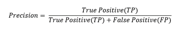
The most desirable behaviour will identify real true positives without introducing too many false positives.
Recall on the other hand looks at how many actual occurrences of the event did the AI model fail to identify (the burglars have made off with the jewellery and the smart device thinks it’s listening to the cat).
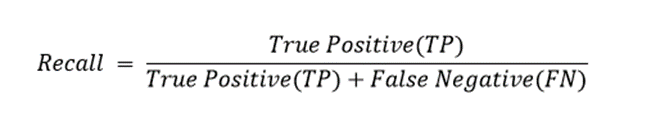
A high recall rate indicates that key occurrences of the target event are not being missed.
For a more complete description of these terms see this resource [https://developers.google.com/machine-learning/crash-course/classification/precision-and-recall]
Effective performance of a model is a balance between these two metrics; the model needs to be able to make a decision that may not be perfect, and the user (human) may need to apply some constraints to how that decision is used.
Use cases – what question are we trying to answer?
The use case for the machine learning model will usually determine how accurate it needs to be and to what degree false positives, or false negatives can be tolerated.
The smart home example is a use that is becoming more ubiquitous and provides some comfort to property owners, but other applications can be of a more serious nature. Companies like ShotSpotter use acoustic sensors to detect gunshots and dispatch local law enforcement. The technology has the potential to be lifesaving, but it is not without controversy.
[https://www.shotspotter.com/shotspotter-responds-to-false-claims/, https://www.datasciencecentral.com/shotspotter-ai-at-its-worst/ ]
The use case will in most applications depend on the question that the machine is being asked. A very specific question can be answered specifically. This is where machine learning excels, repeating a well-defined task over and over. However, a more general question requires a more nuanced approach and a more comprehensively trained model.
Consider the following questions:
1. Was that the sound of glass breaking?
or
2. What was that sound?
The first question has a specific frame of reference, and the decision-making process only needs to evaluate if this is glass or not glass. A well-trained model with a comprehensive library of sample data would most likely produce reliable results.
The second question however requires far more “intelligence” to be included in the AI model. The machine must be able to categorise a sound into one of many choices, based on some training and then make a decision about the most suitable option for the classification. This requires much more extensive training data and subsequently leads to a more involved process.
The following visual example illustrates this idea and the complexity that can be involved in automating a decision-making process. Much like in acoustics, introducing some background noise can quickly make things more complicated.


Machine learning techniques for audio analysis
The first technical step in a machine learning task is feature extraction. This is the process of analysing the input to find some high-level indicators that can be used to identify these inputs under one or more headings. Of course, in the case of acoustics we are most commonly talking about audio files and features of a sound signal. Feature extraction allows an ML algorithm to identify and learn the key aspects of characteristic audio samples such as speech, music, specific events, gender or emotion, depending on the granularity of the application.
Audio feature extraction is usually performed on short time frame segments, usually of 10 to 100ms duration. So rather than analyse a full audio sample of say 30s, much shorter segments are analysed separately, and the results can be averaged across the full recording. There are a few reasons for this approach, but of most relevance is the robustness that it delivers for an audio classification model.
This windowing technique splits the audio sample into a number of short segments. The short frame sizes also allow for better separation between audio events which might otherwise be conflated in one long audio sample. Analysing a signal in short windows helps to account for the fact that the acoustic signal is always changing. Short duration events and more salient features in the audio sample can be detected more accurately using this approach.
Any audio file contains a wealth of information that can be used to detect patterns and label content. The analysis techniques used to extract these features can vary depending on the application i.e. speech recognition, music genre identification or more general audio scene classification. The features that are computed for each individual segment can either be time-based features, based on the raw audio signal e.g. wav file, frequency domain features from a Fast Fourier Transform (FFT) or cepstral features based on the cepstrum of the signal. The short audio segments sacrifice resolution in the frequency domain (less samples for an FFT), but they add flexibility to the technique by allowing larger audio samples of varying lengths to be analysed in micro segments, with the average results being used to classify the full audio file.
Audio signal features
Energy – assuming all audio recordings are normalised, the RMS amplitude can give an indication of the overall loudness of the file. Rock music will usually have a higher RMS amplitude than classical music, while angry or emotional speech track may be higher than a calm conversation.
The zero crossing rate is extensively used in music genre and speech recognition analysis. The zero crossing rate measures how many times the waveform crosses the zero axis within an audio frame. This feature is used good to effect in music recognition applications, with highly percussive genres like rock and pop generally having a higher zero crossing rates. The metric can also be used a rough indicator of the presence of speech in an audio track, with speech segments having distinguishable characteristics when compared to instrumental music frames.
Spectral features
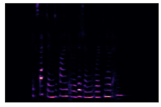
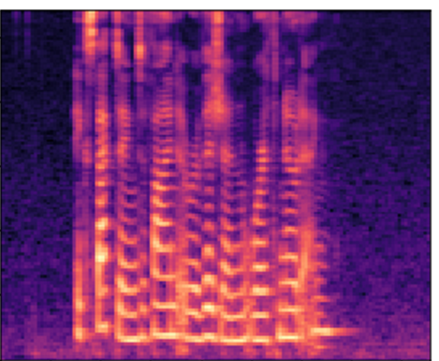
Where machine learning approaches differs from more traditional acoustic signal analysis is the ability to leverage the extensive work that has been done in image recognition to identify sounds based on a spectral image of the signal i.e. a spectrogram. Converting an audio track into a frequency domain image file allows the use of highly sophisticated image processing tools to develop faster and more efficient ML models. In essence, the machine is “looking” at the signal and deciding what the spectral image represents.
Representing perceptual information
In this approach, sound samples are converted into visual representations of the most important information in the signal before being processed in the AI model. This additional step of extracting the most relevant data involves the use of the Mel Scale to highlight perceptually important features.
The Mel Scale accounts for the human ear’s ability (or inability) to distinguish between changes in frequency. In the same way as we use the decibel scale to represent changes in amplitude with more relevant steps, the Mel Scale represents changes in frequency in perceptually relevant steps.
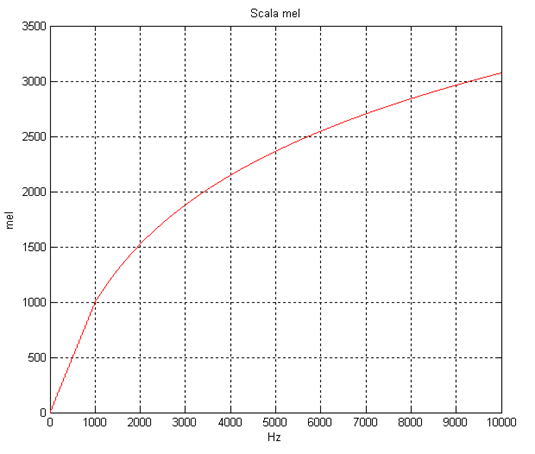
So rather than using a spectrogram as an image of the signal, most audio classification techniques use the Mel frequency approach to “zoom in” on the perceptually relevant information within the spectrogram. An additional step of calculating the cepstral coefficients may also be used to give a representation of the short-term power spectrum, resulting in a bank of Mel Frequency Cepstral Coefficient (MFCC) values which are used to represent the signal.
Model development and detection
These Mel frequency spectrograms are then fed to a Convolutional Neural Network (CNN), a classification technique which is widely used in image processing and recognition applications. This type of algorithm is highly effective at analysing and weighting the content of images and also requires less pre-processing than alternative classification approaches [reference here]. The CNN extracts the features of the spectrogram which are relevant for machine learning model classification. The labels applied to the original audio training files are then associated with these feature sets. When the AI model detects the occurrence of a particular feature set in any subsequent audio stream (from the averaged results of the microsegments) then the associated label can be applied.
Instrumentation and monitoring equipment
So, what does all this have to do with instrumentation and monitoring equipment? Well, with the proliferation of smart devices and the increase in portable computing power, far more of this computation is now possible in the field. This is known in the sensor network industry as “processing at the edge,” where most of the data processing is done on a device in the field.
The processing intensive steps of training and developing audio recognition models can be done using cloud computing resources or high-powered computers, but the final AI models that are used can be relatively lightweight in computing terms. This means that the hardware that is performing the audio recognition does not need particularly large amounts of power or resources to simply capture an audio stream and classify the sounds. Furthermore, all major chip manufacturers are now including artificial intelligence hardware in their future roadmaps. This hardware accelerated AI will perform these classifications faster and more efficiently than current versions, further reducing the barriers to wide scale deployment of the technology. This gives audio professionals the opportunity to develop and deploy networks of sensors, appliances or sound level meters that can not only measure sound, but also understand the context of the soundscapes they are measuring.
A short search in any patent listing can reveal a range of possible applications from lifesaving medical devices to coffee machines that can hear when the washing machine stops. As the technical barriers continue to fall, audio recognition will no doubt become even more ubiquitous.
Frequency response and microphones
For use cases with high accuracy requirements consideration should be given to how the training audio data is captured and how that compares to the audio device used in the field. For example, if an AI model is trained using audio files sampled at 48 or 96kHz and recorded with studio quality microphones in an anechoic chamber then the resulting audio will sound impeccable. If the resulting AI model were deployed on a device with a low-cost microphone, housed inside an appliance, mounted in a dashboard or carried in one’s pocket, then the quality of the measured audio in the field could vary significantly. The influence on frequency response by a change of microphone or a device housing cannot be neglected where computational resources at the edge might be constrained. Model development and training should either be done on representative audio samples or should be tested extensively for robustness to field conditions.
While the technical barriers to developing a sensor and ML tools are certainly dropping, there are sensitive applications in healthcare, condition monitoring and security that will always require the expertise of a seasoned acoustician to use their own ears and make sense of the signals.
And for those among you who get the sense that your phone might be listening to you… the answer is almost certainly yes.